In this post, I walk through an improved FPGA hashtable design, following on from my earlier post. Unlike that post, I’ll mostly focus on the hashtable design, rather than using it to build an actual networked key-value-store.

I also explain my formal verification based development methodology, which allowed me to gain a lot of confidence in the design before even writing a single test.

The SystemVerilog code for the hashtable implementation is available here.

Background

Hashtables are useful data structures, whether you’re designing software or hardware. In my earlier post, I walked through the design of a basic one based on Cuckoo hashing. As that post describes, looking up keys is very simple with Cuckoo hashing - just check each table for the key of interest. The main innovation of that post was the idea of a “cuckoo loop”, for handling the more difficult insert operation.

However, the design suffers from a couple of major limitations that limit its practical utility:

1. If there is an insert or modification in progress, all subsequent operations are stalled until that operation completes. For inserts, that is an unbounded amount of time.
2. The logic depth, at 12 levels, is fairly deep, and that’s for only 32 bit keys and values.

(1) limits the frequency of operations we can perform on the table. If an insert operation is in progress, we must stall everything and wait.

(1) also limits us to performing only one insert operation at a time. However, a Cuckoo hashtable is made up of multiple independent RAMs, so we should, in principle, be able to perform multiple insert/eviction operations in parallel in a pipelined fashion, reducing the average time to insert a key. To do this, we’d need to support multiple inserts/evictions in flight as well as forwarding the evicted values to lookups occurring simultaneously.

(2) prevents us from operating at higher clock frequencies and makes it harder to reuse the design in larger systems as it may cause issues with timing closure.

I decided to create an improved hashtable that fixes these flaws. The next section explains the top level operation of the new hashtable and how the limitations of (1) are overcome with an interface where in-flight inserts do not block other operations. The final section presents the synthesis results and despite all the forwarding, the logic depth is a more healthy 8 levels.

Design goals

The hashtable is implemented in on-chip RAM and is intended to hold a few tens of thousands of key-value pairs per table. This means that a single table will occupy a few tens of UltraRams.

Modern Xilinx FPGAs can contain hundreds of UltraRams, so to utilise all of them, something like hash sharding within a single FPGA could be used as long as the shards remain balanced. Note that the biggest FPGAs only contain ~50 Megabytes of on-chip SRAM, so storage is very limited compared to hashtables that live in DRAM, however you structure things.

The top level block diagram of the hashtable is given in the figure below.

Unlike lookups, inserts into a cuckoo hashtable are not constant time, and thus takes a variable number of cycles in hardware. To accommodate this, the hashtable outputs a busy signal when it is currently unable to accept an insert. If the user asserts the insert signal and the hashtable is not busy, then the key-value-pair is accepted on that cycle.

Of course cuckoo hashtable inserts are not constant time operations, so the insert operation does not actually complete immediately. But the hashtable’s internal forwarding network gives the illusion that it does.

The waveform below illustrates an insert operation. Initially the insert signal and busy signals are both asserted (cycle 0), so no insert takes place. Once busy is deasserted (cycle 2), it accepts the value to be inserted. If we to do a lookup just one cycle later (cycle 3), it would return the inserted value (cycle 5, after a configurable pipeline depth, more on that later).

Lookups, modifications, and deletes are constant time operations for cuckoo hashtables so are not subject to backpressure in the form of a busy signal. In fact, you can launch these operations at any time regardless of the value of the busy signal and they will be serviced immediately. This ‘non blocking’ feature, where the constant time operations are serviced immediately, regardless of in-progress inserts, is an important feature of this hashtable.

Modifications and deletes are always preceded by a lookup operation to find the location of the key in the table (if it exists). One or two cycles after the lookup is initiated (depending on the configurable pipeline depth), the presence and value information associated with the key is returned. Then, on the same cycle that the value is returned, you have the option to modify the value or delete the key-value-pair entirely. This means that the new value can depend on the old value. You can perform atomic read-modify-write operations on the value associated with a key.

Lastly, the waveform below shows a read-modify-write operation. The key is assumed to already be present in the hashtable at the beginning of the waveform. The lookup is initiated in cycle 1 (regardless of the busy signal, which isn’t shown), and two cycles later (the configured pipeline depth), in cycle 3 the presence and value information is made available. User logic outside the hashtable increments the value and asserts the modify input to tell the table to update it’s copy of the value, also in cycle 3.

The waveform illustrates a slightly unintuitive feature of the design. Conceptually, the modification is deemed to have occurred in the cycle that the original lookup took place, even though the new value is not made available to the hashtable by user logic until two cycles after the lookup. In the waveform, the same key is looked up again in cycle 2. When it’s value returned by the hashtable in cycle 4 it is the new value. This allows back to back modifications of a value on consecutive cycles.

Design

At a high level, the design is based on the “cuckoo loop” idea explained in more detail in my earlier post, and shown in the diagram below.

Key-value pairs to be inserted are injected into the columns, which consists of RAMs, insert/eviction logic, and lookup/modify logic. If there was already something present in its slot (ie at the address of the hash of it’s key), it is evicted and injected into the next column in the loop, where a different hash is used. Key-value pairs make their way around the loop until they all settle in a free slot, which will happen eventually unless the table is nearly full.

The core of the design is the “column” in the figure above. It processes incoming inserts and outgoing evictions for a single RAM. It also handles lookups, modifications and deletes for keys, if they are in the RAM it’s responsible for. This is also the part that makes the “non blocking” behaviour possible, and is the main difference from my earlier design.

A couple of observations, which I will elaborate on below:

1. The write address is just a delayed version of the read address. It’s delayed by NUM_PIPES cycles, where NUM_PIPES is the configurable pipeline depth of the design. But in the diagram, and the explanation below, I’ll take NUM_PIPES to be 1 to simplify the explanation.
2. The RAM’s read address port is sourced from one of three values - incoming evictions, delayed evictions (marked *), and lookups.

(1) is required for the writeback step of modification and delete operations. As in the waveforms above, the writeback operation is always delayed by NUM_PIPES cycle from the original lookup request. This must be the case because initially we don’t know which column the key resides in, or if it resides in the table at all. So, we must wait for that information before we can do the writeback.

Unlike modifications, evictions don’t require the write address to be a delayed version of the read address. We could write and read the same location on the same cycle to simultaneously write the incoming evicted/inserted value and read the value we are replacing to be re-inserted downstream. However, it turns out that the write address logic, and the overall design are simplified if we apply a matching delay to eviction writebacks, even though we don’t strictly need to.

Consider the case where in cycle 0 a lookup/modify operation is initiated. In cycle 1 we are performing the writeback step of the modify. But, suppose there is also an incoming eviction. The write port is occupied by the writeback from the modify in cycle 0, so where will the evicted value go? A simple solution is to always apply a matching delay to the eviction write so that it happens in cycle 2.

Of course, we also need to consider read address port conflict where a lookup and eviction occur simultaneously in cycle 1. Since it is a design goal that lookups are always serviced immediately, we give the lookup priority. This is part of the reason for (2) above. If an eviction was in progress, we need somewhere to put it so that it is not lost while the lookup is being performed. We conveniently reuse the delayed eviction register in the figure above for this and mux this into the read port in cycle 2. This time we keep the delayed eviction in the register for another cycle and write it back in cycle 3.

We can keep the delayed eviction from cycle 2 around until cycle 3 because we know there will be no incoming eviction from the previous column in the loop on cycle 2. A lookup is performed in all columns simultaneously so the previous column in the loop was also performing a lookup in cycle 1, which means that it cannot have an outgoing eviction in cycle 2.

The above description only touches on the simplifications afforded by delayed evictions. They also simplify the forwarding logic between the insert/eviction process and lookups/modifications considerably. More concrete details can be found in the heavily commented source.

Formal verification

One of the main ideas I wanted to convey in this post is the power of formal verification for designing digital logic. I used a limited form of formal verification called bounded model checking, which unrolls state transition system of the design for a fixed number of steps, N, and checks whether an assertion is violated during those steps. So, it is not a full proof of correctness but rather a proof that no bugs occur in N clock cycles. Bounded model checking is supported by the excellent open source symbiyosys tool.

If the design is complex, but the top level specification of its functionality is simple, then it’s probably a good candidate for formal verification. For example, consider a hashtable. The design presented in this post consists of logic to store evicted keys and values, writeback logic for modifications, forwarding networks, and so on. Its implementation is fairly complex, but at a high level, it is straightforward to specify what it actually needs to do. Roughly:

• If a key has not been inserted, lookups will not succeed
• Once a key-value-pair has been inserted, subsequent lookups to that key return the value associated with that insert
• Modifications and deletions update the value for that key accordingly and subsequent lookups return the correct value

A slightly simplified spec is given, below. The spec is brief, and therefore likely to express the actual functionality you want. The whole idea is to have a spec that is much simpler than the implementation. However, it still deserves some explanation.

module formal (
    input logic       clk,

    //The SMT solver can set these arbitrarily
    input logic       insert,
    input logic [7:0] ins_key,
    input logic [7:0] ins_value,

    input logic       lookup,
    input logic [7:0] key
);

logic       valid;
logic [7:0] value;
logic       busy;

//Instantiate the DUT
kvs kvs_inst (.*);

//Signals prefixed with f_ hold the state of the key-value-pair we are tracking
//f_key is arbitrary, but constant for the duration of the run
(* anyconst *) logic [7:0] f_key;
               logic       f_valid = 0;
               logic [7:0] f_value;

//Track the value associated with our formal key
always @(posedge clk)
    if (ins_key == f_key && !busy && insert)
        //It is illegal to insert a key that is already inserted.
        assume(!f_valid)

        f_valid <= 1'b1;
        f_value <= ins_value;
    end

//Track if we did a lookup in the previous cycle
logic f_past_lookup = 0;
always @(posedge clk)
    f_past_lookup <= lookup && key == f_key;

//Assert that the presence information and value are correct following a lookup
always @(*)
    if (f_past_lookup) begin
        assert (f_valid == valid);
        if (f_valid)
            assert (f_value == value);
    end

endmodule

The code above uses a technique I first heard about on Dan Gisselquist’s blog, and is better explained there. In short, the verifier is allowed to pick a single arbitrary key to track for the duration of the run. It generates an arbitrary sequence insertions, modifications and lookups for a range of keys. It tracks the value associated with the key it chose to track, and if the hashtable returns the wrong value, it fails an assertion. Since the key was arbitrarily chosen in the first place, the property applies to all keys.

Designing with formal verification is a lot like peer programming with a truly brutal peer. They spot even the slightest mistake immediately. They present you with a counterexample trace that shows you exactly what went wrong. However, they are nice enough to make sure that the counterexample traces are short, so you don’t have to keep traces thousands of cycles long in your head when trying to understand the bug.

The last point is worth reiterating. Had I been using conventional randomised testing, many of the bugs would have been found in traces thousands of cycles long. It is exceptionally difficult to understand how your design went wrong in a thousand line trace. With bounded model checking, you get the shortest trace that leads to a spec violation. Most of the traces I was debugging while developing this hashtable using bounded model checking were less than 10 cycles long.

As mentioned above, bounded model checking is not a full proof of correctness, it only tells you that there are no bugs within N cycles. In this case N=12, since that’s the depth that the formal tools were able to reach with my design after running for about a day. That doesn’t sound like much, but it is still quite a strong guarantee when you consider that the tools are considering all possible inputs to the design. The formal tools found all kinds of issues in the forwarding logic that I never would have considered. And, when I did implement a traditional randomised testbench (below), that was not able to find any remaining bugs.

For a full correctness proof, you need k-induction, which is also supported by symbiyosys. That is something I’ll look at in the future.

The actual heavily commented spec is here.

Testing (sim and real world)

In addition to performing bounded model checking, I have implemented a traditional randomised testsuite. While the bounded model check gives me a lot of confidence in the design, it only shows correctness for a bounded number of cycles. Also, while the spec is short and simple, it’s still human written code and might contain mistakes.

The testsuite, which uses the wonderful verilator as the simulator, is basically the same as described in the testing section of my original blog post, except that it’s written in Rust, not Haskell.

It randomly generates a sequence of hashtable operations and feeds them to the simulated hashtable and a software mirror hashtable, and checks that all lookup operations performed by the design return presence and value information that matches the mirror.

In principle, if you run this for long enough it will hit all the corner cases. However, to gain more confidence in the design, the testsuite tries to generate sequences of operations that will hit nasty corner cases with higher probability than random chance.

For example, I have tried to exercise the forwarding logic as much as possible. To do this, I keep a queue of recently inserted, modified or deleted keys, and perform subsequent modifications or deletes on these keys more often than would happen if keys were chosen at random. Note that a fair bit of effort went into exercising these testcases, whereas with the formal properties, you get these for free.

Load factor

The formal tests say that after any sequence of inserts, modifications, and deletes, a subsequent lookup will always return the correct value. However, they don’t prove that the hashtable achieves a good load factor. In fact, if the hashtable just asserted busy continuously (thus preventing any inserts from happening), then it would actually satisfy the formal properties.

The traditional randomised tests allow us to run for many cycles and load up the hashtable and check that it achieves the expected load factor. A cuckoo hashtable with four RAMs should be able to achieve a load factor in excess of 90%. The waveform below shows a zoomed out view of the beginning of the test where the framework inserts 15000 random key-value pairs, which, with a table size of 16384, represents a 91.5% load factor.

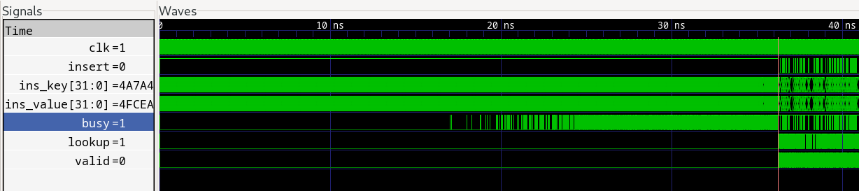
We can see that the hashtable is able to insert all key-value pairs, but as it fills up, it takes more time to insert each pair. It is able to insert almost half of them without any backpressure (busy is low), but as it gets closer to being full, it asserts busy frequently. This is expected, since as the table fills up, more evictions must be performed for each insertion.

This also highlights another nice feature mentioned above - there is insert/eviction parallelism. Each RAM performs an eviction every clock cycle. Thus, if you have N RAMs, you can perform N evictions in parallel. This improves eviction performance when the table starts to fill up.

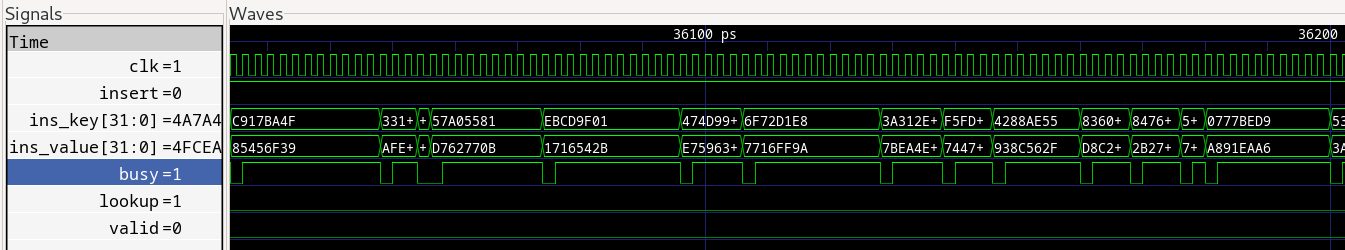
The waveform below is a zoomed in version of the end of the loading-up phase when the hasthable is ~90% full. You can see that, in contrast to the beginning, the table is busy for several cycles after each insert, as expected due to the required evictions. If this is an issue, then you could use a bigger table and operate at a lower load factor, or use more tables to take advantage of the higher achievable load factor as well as increased insert/eviction parallelism.

It’s worth noting that the randomised testsuite didn’t find a single bug, and all tests passed first time. Ie, whatever bugs the randomised test would have caught, the bounded model check caught first.

There is also a demo design here that implements the hashtable on a real world FPGA. Commands can be sent to the FPGA over JTAG from within the Vivado GUI using Xilinx’s VIO core. The outputs of the hashtable can also be captured in the GUI using Xilinx’s ILA core.

Implementation

The implementation report below is for a single hashtable with 64 bit keys and values and consisting of four columns and is capable of storing 16384 key-value pairs. The source for the standalone design, made for the purpose of checking timing, can be found here. Larger memories meet timing too at around the same frequency if the pipeline depth is increased.

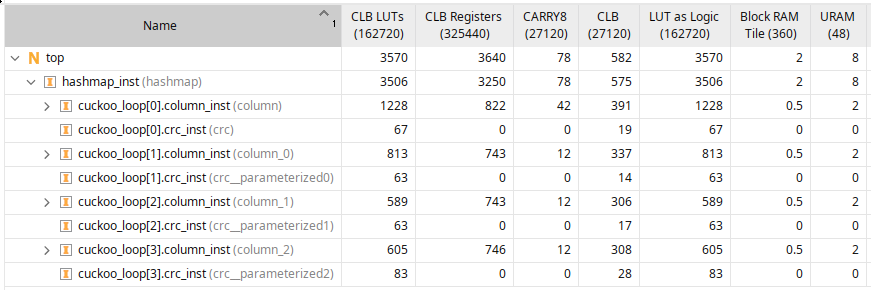
As expected, 8 ultrarams are used - 2 for each column - where one is used to store the 64 bit key, and one is used to store the 64 bit value. Block RAMs are used to store the valid bit. Most of the logic and CARRY8s are used for the forwarding network, and most of the registers are used for the pipeline stages.

The maximum logic depth is 8 for this 64 bit key and value case, and the design meets timing comfortably at 350MHz, if synthesized standalone.

Future work

The design has a configurable pipeline depth, which places pipeline stages after the RAMs. Two stages is good for small tables, as demonstrated above. However, the matching and bypass logic is not pipelined, and that is needed to operate at frequencies >350MHz, or within FPGAs that are filling up.

This post was focussed on the design of the hashtable itself. But it’s also interesting to think about what you could build with it. With a high speed (10G+) Ethernet MAC, and some network packet parsing code, the hashtable could be hooked up to a network to build a networked key-value-store providing exact match searches.

As mentioned above, to scale the design to use the whole chip, multiple hashtables could be implemented on a single FPGA, and hash sharding could be used to distribute keys amongst individual tables. The tables operate in parallel and each table is capable of 350 million operations per second, so as long as the operations are distributed roughly evenly amongst the sharded tables, the combined system could service billions of operations per second. Of course, you would need an FPGA with several high speed Ethernet connections to communicate operations at this rate, as well as a complex routing network to connect each transceiver to each hashtable.