This post is about my entry in the Reactive Synthesis Competition. I wrote it several years ago, and, as of this year, it doesn’t even win its track anymore. However, I recently saw reactive synthesis mentioned in the SymbiYosys docs and got excited because that means that someone outside of academia is possibly interested in reactive synthesis. So, I thought I’d write a very high level blog post introducing reactive synthesis and my solver.

Specifically, I will be talking about the safety track of the reactive synthesis competition. The reactive synthesis competition is an academic competition where people submit solvers for a particular problem (described below) and the solvers are run to see which one can solve the most problems in a given amount of time. The objective is to synthesize a controller (or just determine if one exists in the realizability track) for a finite state safety game. Exactly what a safety game is, and how it is solved, is described below.

The Problem

I think the problem is best described using a sequential digital circuit such as the one in the diagram below. The circuit contains of a set of state registers that are updated on each tick of an single implicit global clock. The next-state values of the state registers are provided by the block labelled “System”, which only contains combinational logic. There are three inputs to the “System” block:

1. The values of the state registers in the current cycle (S),
2. A set of boolean “uncontrollable” signals provided by the environment (U),
3. and, a set of boolean “controllable” signals driven by a controller circuit (C).

And, two outputs:

1. A boolean “BAD” signal that goes high if the circuit has reached an unsafe state,
2. A vector of boolean signals (S’) that determine the values of the state registers in the next cycle.

Given U, C, the set of state variables, and the system, it is the job of a solver entered in the reactive synthesis competition to synthesize the boolean logic for the controller. A correct controller, when placed in the circuit above, ensures that the boolean output variable BAD never goes high for any execution of the system.

The controller circuit has access to the uncontrollable inputs as well as the state registers. It may be purely combinational or it may contain its own state registers. However, it turns out that, at least for safety games (described below), if any controller exists, then so does a controller without state registers.

Safety games

This is called a game because you can think of the controller as playing a game against the environment, where, on each tick of the global clock, the environment makes a move by setting the uncontrollable inputs. The controller must react with a matching move (setting the controllable signals) to ensure that BAD never goes high, and, additionally, that future executions of the system can not lead to a state where BAD goes high, whatever the environment does. We could say that we are safe when BAD is false. Our goal is to always be safe, which is why this type of game is called a safety game. Note how this differs from a liveness condition where something is required to be true eventually.

We can make this more explicit with an example, given below. The state space of the game consists of two state registers: X and Y, drawn on the two axes. There are a total of 4 states, each corresponding to a valuation of each of the state registers. Initially, the game begins in the top left corner, corresponding to the valuation X=0, Y=0. The game progresses according to the values of the C and U signals. The notation on the transitions is E/C, i.e. the transition labelled 0/1 will be taken if E has value 0 and C has value 1. If there is no corresponding label, the game stays in the same state. “X” means don’t-care. In this example, in the black state the BAD output variable will always be high. The controller must therefore ensure that no execution of the system can ever reach this state. As an exercise, see if you can express this example (System in the diagram above) as a sequential digital circuit, perhaps in Verilog. Hint: it must have two boolean state registers, X and Y, two boolean input variables, E and C, and output the next-state values of the two state registers as well as the BAD signal.

Note that the controller has full visibility of all the state registers. This is called a complete information game as opposed to a partial information game where only a subset is visible. Additionally, the combinational logic of the system is an input to the synthesis problem, so the synthesis algorithm knows exactly how the system will behave for all inputs.

There is a controller for this example system that ensures execution avoids the black state indefinitely. Starting from the initial state, if the environment sets E = 1, the controller can do whatever it wants. If the environment sets E = 0, the controller must avoid the transition to the top right state. If execution enters the top right state, then all the environment has to do to win is set E = 1 in the next transition (if it set it to 0 then the state would be unchanged, see above) - theres is nothing the environment can do - execution will inevitably end up in the bad state.

Fortunately, the transition to the top right state can be avoided. All the controller has to do when E = 0 in the top left state is to set C = 0. This directs execution to the bottom left state and there is no danger of entering the bad state (provided the controller keeps doing the right thing in the future).

As an exercise, see if you can express this controller as a digital circuit. Hint: it is purely combinational, has two boolean state inputs X and Y, another boolean input from the environment E, and a single boolean output C.

How it is solved

Safety games are solved by an iterative algorithm, which I will demonstrate on the example above. Obviously, the black state is losing. If execution ever enters that state, BAD = 1 and the game is lost. Starting from the black state, we find other states from which the environment can force the game into the black state in one step. Then we perform this operation again to find the states from which the environment can force the game into the black state in two or less steps. By iterating this, we eventually find all of the states the environment can win from. If the initial state is one of these, then the game is not winnable by the controller. Otherwise, it is winnable.

To find the set of states from which the environment can force execution into the losing states, we use an operation called the controllable predecessor. The controllable predecessor considers each losing state and checks if there exists an environment action such that, for all controllable actions, execution ends up in a losing state.

Consider the controllable predecessor applied to the losing set containing only the BAD state in the example above. If the environment plays a 1, then, there is nothing the controller can do, execution will always end up in the bad state. So, the top right state is added to the losing set. Consider another iteration of the controllable predecessor. The BAD state is only reachable by the top right state, and that is already in the losing set, so we only have to consider moves that take execution to the top right state. However, there are no such moves that guarantee that. The only candidate environment move is to play a 0. However, the controller can thwart this by also playing a 0, steering execution into the bottom left state instead. The algorithm terminates because there are no more losing states to discover and the final losing set is just the two right states. As this does not include the initial state, the game is winning for the controller.

Note that this algorithm always terminates. Every step either adds at least one new state to the losing set, or, there are none to add and the entire losing set has been found. Since there are only a finite number of states in the game, states will only be added to the losing set a finite number of times, and the algorithm will not iterate forever. When the algorithm terminates the state space of the system will be partitioned as in the diagram below. Some subset of the state space will be BAD. Another possibly empty subset, which does not intersect with the BAD set will be winning. The remaining states can be forced into the BAD state by the environment so they are losing. Finally, if the initial state is part of the winning set, the controller wins the game. In the diagram below, this is the case, so the controller wins.

Once you have found the complete losing set you can use it to generate a controller. If execution ever enters the losing set, then it is possible for execution to enter a state where BAD = 1 regardless of what the controller does. All the controller has to do is keep execution out of that set, or, equivalently, keep execution in the winning set. For each state not in the losing set, and for each assignment to the environment controlled inputs, there exists an assignment to the controller signals that keeps us out of the losing set, otherwise, by definition, the state would be in the losing set. The controller just has to make sure to set the controllable signals appropriately in those states.

In the example above, the losing set is comprised of the two rightmost states. When execution is in the top left state, the controller has to set C = 0 when E = 0 to avoid entering the losing set. When execution is in the bottom left state, the controller is free to set C to anything. As long as these rules are followed, and execution begins in the top left state, execution can never enter the losing set and there’s no possibility of BAD equalling 1. The strategy is only defined for the leftmost two states (the complement of the losing set) because, as long as it is followed, execution will remain within that set.

Symbolic solving

The state machine above has 2^n states, where n is the number of state registers. Traversing state machines in this way quickly becomes intractable as n grows larger. Instead, we can represent the state machine and the winning set of states symbolically, a technique borrowed from model checking. Instead of keeping some kind of set datastructure containing the winning states, which themselves are valuations of all state registers, we represent the set using a propositional formula over state registers that is true iff the state is in the set. In practice this is much more compact than explicitly representing the set.

As an example, consider the top right state above, x=0, y=1. We would represent a set containing only this state by the equation “not x and y”. Consider the set containing the two states on the right. We would represent this set simply as the equation “y”. Note the absence of “x” in the formula. You can see how, as the number of state grows, in many cases, this representation becomes more concise.

We need a datastructure to efficiently represent these propositional formulas. We also need to be able to perform logical and quantification operations efficiently. Binary decision diagrams are a perfect fit.

Binary decision diagrams

A binary decision diagram is a directed acyclic graph with a root and two leaf nodes (the square ones). The figure shows a binary decision diagram representing a propositional formula over 3 variables: x, y and z. The circular nodes represent variables and the square nodes, or terminal nodes, represent the outcome of the function. Terminal nodes are labelled either 1 or 0. Given a valuation of X and Y, we can evaluate the function by starting at the root and taking the solid edge if the variable represented by the node is assigned to True in the valuation and taking the dashed edge if the value is assigned to False. When we arrive at a leaf, that leaf holds the value of the function for the given valuation.

If we impose some conditions on the structure of the graph we get a remarkably compact data structure for representing propositional formulas called a reduced ordered binary decision diagram (ROBDD). You can read all about ROBDDs here.

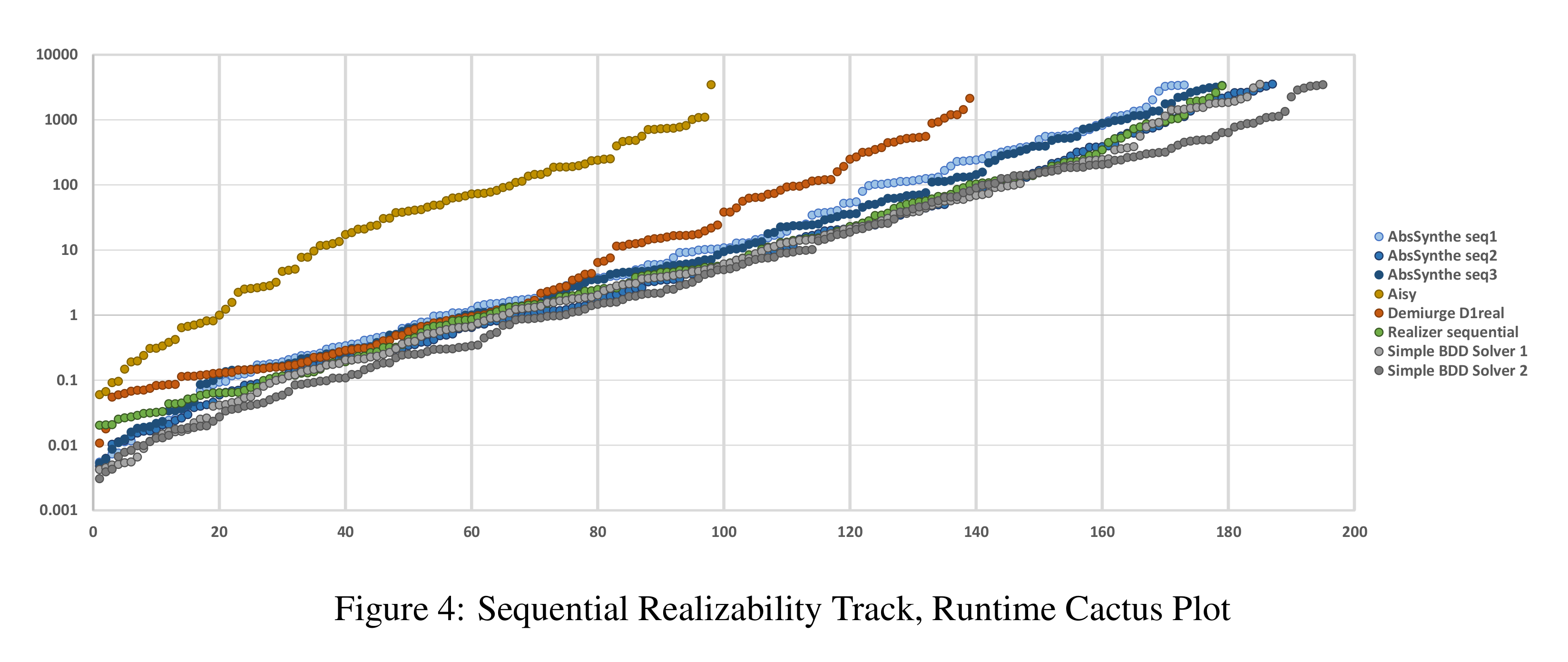
Results

Combining the iterative algorithm above, and BDDs for representing sets of states results in a remarkably efficient solver. In fact, this is how most of the competitive solvers in the Reactive Synthesis Competition are implemented. The results for the sequential realizability track of the 2015 competition (report available here) are given in the graph below. One of my solvers, Simple BDD Solver 1, uses only this algorithm and was placed third that year. There are also some improvements that can be made upon the basic iterative algorithm. My other solver, Simple BDD Solver 2 adds an abstraction-refinement loop on top of the basic iterative algorithm. With this improvement, it won the sequential realizability track. How that works might be the subject of a future blog post.