In this blog post I’m going to give a demo of my sdr library. SDR stands for software defined radio. The library is mostly written in Haskell and is available on Hackage as the (imaginatively named) sdr library. I will be using it to build an FM broadcast band receiver.

Software Defined Radio

Usually, radios are implemented using analog components. With software defined radio, signal processing is implemented on a computer processor instead. This means that by simply changing the software, provided your CPU is fast enough, you can have any kind of radio.

You still need some hardware to digitise the signal coming from the antenna. Specifically, it must filter out unwanted signals, mix the wanted signal down to a lower frequency and then digitise it with an analogue to digital converter (ADC).

RTL-SDR

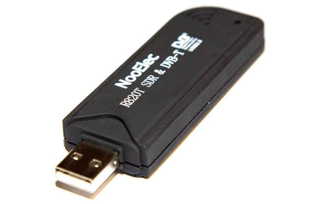
You might expect such hardware to be niche and/or expensive. However, a few years ago, an undocumented mode was found in a cheap TV tuner chip that does exactly what we need. These chips are abundant and can be bought for only US $20. There is loads of cool stuff you can do with one and its also worth checking out the reddit.

Peering into the Broadcast Band

We’re going to build an FM receiver with one. The rtl-sdr is tunable from 24 to 1766 MHz. Fortunately, the FM broadcast band (88 - 108MHz) lies in that range. The rtl-sdr allows us to filter out a 1MHz chunk of that spectrum and mix it down down to baseband.

Lets give it a go. Using the sdr library, we can configure the rtl-sdr to select a chunk of frequencies, take the fourier transform of the incomimg data, and plot a spectrogram.

import Control.Monad.Trans.Either
import Data.Complex
import Foreign.C.Types
import Control.Monad

import Pipes as P
import Pipes.Prelude as P
import Data.Vector.Storable as VS hiding ((++))
import Data.Vector.Generic as VG hiding ((++))

import SDR.Util as U
import SDR.RTLSDRStream
import SDR.FFT
import SDR.Plot
import Graphics.DynamicGraph.Waterfall
import Graphics.DynamicGraph.Util

main = eitherT putStrLn return $ do
    res <- lift setupGLFW
    unless res (left "Unable to initilize GLFW")

    let fftSize  =  8192
        window   =  hanning fftSize :: VS.Vector Double
    str          <- sdrStream (defaultRTLSDRParams 91600000 1280000) 1 (fromIntegral $ fftSize * 2)
    rfFFT        <- lift $ fftw fftSize
    rfSpectrum   <- plotWaterfall 1024 480 fftSize 1000 jet_mod

    lift $ runEffect $   
            str 
        >-> P.map (interleavedIQUnsigned256ToFloat :: VS.Vector CUChar -> VS.Vector (Complex Double)) 
        >-> P.map (VG.zipWith (flip mult) window . VG.zipWith mult (halfBandUp fftSize)) 
        >-> rfFFT 
        >-> P.map (VG.map ((* (32 / fromIntegral fftSize)) . realToFrac . magnitude)) 
        >-> rfSpectrum 

There are several important things to note in this code. Firstly, we setup GLFW as we will be using that with OpenGL to render our waterfall plot. Next, we initialize out rtl-sdr device and create pipes which will do various signal processing tasks for us.

The first of these tasks is to stream samples from the rtl-sdr device. We use the sdrStream function to generate a Producer.

We tune to 91.6 MHz because this signal happens to be particularly strong where I live. The sample rate is set to 1.28MHz because that was what I randomly decided.

Samples generated by the rtl-sdr are quadrature sampled. This means that each sample is represented by a complex number. The raw 8 bit samples from the rtl-sdr are the interleaved in-phase and quadrature components of these samples. To transform this interleaved array to an array of complex floats we use the interleavedIQUnsigned256ToFloat function.

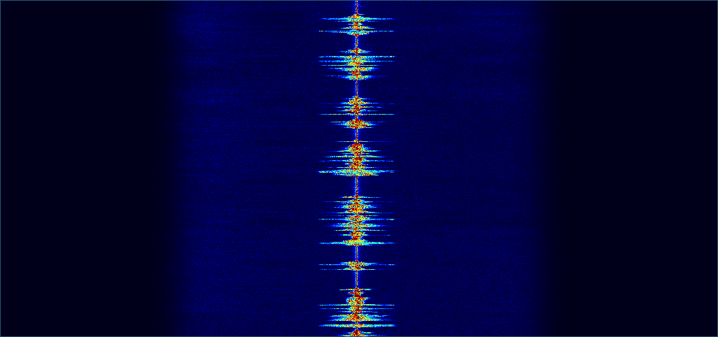
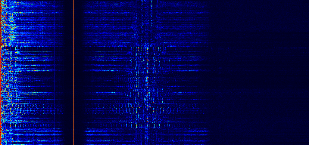
Next, we window the data, take its Fourier transform and then take the magnitude of the result. Finally, we pipe this into the waterfall consumer we created earlier, which displays the data for us nicely:

We can see that there are two stations transmitting in this chunk of spectrum - the strong central one that we will be receiving and a weaker one which we will discard.

Decimation

The first thing our FM receiver must do with the received signal is select only the band we want (the one in the middle) and reject all the others. We can do this with a low pass filter. By removing the higher frequencies, the low pass filter also allows us to reduce the sample rate without introducing aliasing. Reducing the sample rate is called decimating.

First we will just try filtering without the decimation to see what effect it has.

Designing a filter

I plan to decimate by a factor of 8. It’s usually more efficient to decimate in stages, so I will decimate in three stages, reducing the sample rate by a factor of 2 each time. The first thing we must do is design the anti-aliasing filter. Fortunately, the sdr library provides functions to design the filter as well as plot the frequency response so that it can be inspected:

import Data.Complex
import Data.Vector as V hiding ((++))
import SDR.FilterDesign

main = do

    let coeffsDecim :: [Double]
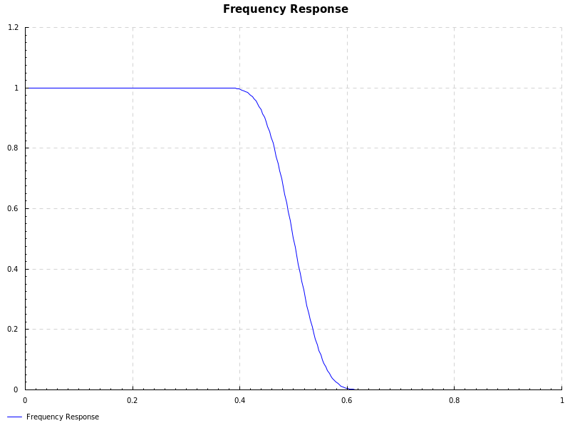
        coeffsDecim =  V.toList $ windowedSinc 45 0.5 blackman

    plotFrequency coeffsDecim "frequency_response.png"

We use the window method of filter design to generate some filter coefficients. Specifically, we request a filter with 45 taps and a cutoff frequency of 0.5 * the Nyquist frequency. If too few taps are used, the filter transitions too slowly into the cutoff region. If too many are used, the filter becomes too computationally expensive. In order to avoid aliasing, we need to remove all frequency components above 0.5 * the Nyquist frequency, which is why we use 0.5 for the cutoff. We observe the frequency response of the filter with the plotFrequency function:

Next, we apply the filter to the incoming signal and plot another waterfall.

let coeffsFilter :: [Float]
	coeffsFilter =  VS.toList $ windowedSinc 45 0.5 blackman
filter <- lift $ fastFilterC cpuInfo coeffsFilter

lift $ runEffect $   
		 str 
	 >-> P.map (interleavedIQUnsignedByteToFloatFast cpuInfo :: VS.Vector CUChar -> VS.Vector (Complex Float)) 
	 >-> firFilter filter fftSize
	 >-> P.map (VG.zipWith (flip mult) window . VG.zipWith mult (halfBandUp fftSize)) 
	 >-> P.map (VG.map (fmap float2Double))
	 >-> rfFFT 
	 >-> P.map (VG.map ((* (32 / fromIntegral fftSize)) . double2Float . magnitude)) 
	 >-> rfSpectrum 

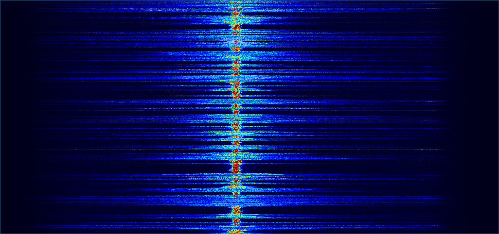
As expected, not only have the signals on either side of the central one disappeared but all of the noise at those frequencies is gone too.

Reducing the sample rate

Now that we have verified that our anti-aliasing filter is working correctly, we can decimate to reduce the sampling rate. We could first apply the filter and then drop every second sample. However, it is more efficient to not compute those dropped samples in the first place. That is what the firDecimator function does in the code below. Note that we decimate by a factor of 2, 3 times, so that we decimate by a factor of 8 overall.

let coeffsDecim :: [Float]
    coeffsDecim =  VS.toList $ windowedSinc 45 0.5 blackman
deci <- lift $ fastDecimatorC cpuInfo 2 coeffsDecim 

lift $ runEffect $   
        str 
    >-> P.map (interleavedIQUnsignedByteToFloatFast cpuInfo :: VS.Vector CUChar -> VS.Vector (Complex Float)) 
    >-> firDecimator deci fftSize
    >-> firDecimator deci fftSize
    >-> firDecimator deci fftSize
    >-> P.map (VG.zipWith (flip mult) window . VG.zipWith mult (halfBandUp fftSize)) 
    >-> P.map (VG.map (fmap float2Double))
    >-> rfFFT 
    >-> P.map (VG.map ((* (32 / fromIntegral fftSize)) . double2Float . magnitude)) 
    >-> rfSpectrum 

And, the result…

As well as reducing the sample rate, this has the effect of zooming in on the frequencies of interest. This is because, since our sample rate has been divided by 8 (from 1280 KHz to 160 KHz), so has the Nyquist frequency.

Decoding the FM Signal

Now that we have selected our band of interest, we can decode the frequency modulated signal. Decoding an FM signal is straightforward. We simply take the difference in phase between the current sample and the previous one as this is proportional to the current frequency. That’s all the fmDemod pipe does.

audioFFT       <- lift $ fftwReal fftSize
audioSpectrum  <- plotWaterfall 1024 480 ((fftSize `quot` 2) + 1) 1000 jet_mod

lift $ runEffect $   
        str 
    >-> P.map (interleavedIQUnsignedByteToFloatFast cpuInfo :: VS.Vector CUChar -> VS.Vector (Complex Float)) 
    >-> firDecimator deci fftSize
    >-> firDecimator deci fftSize
    >-> firDecimator deci fftSize
    >-> fmDemod
    >-> P.map (VG.zipWith (*) window) 
    >-> P.map (VG.map float2Double)
    >-> audioFFT
    >-> P.map (VG.map ((* (32 / fromIntegral fftSize)) . double2Float . magnitude)) 
    >-> audioSpectrum

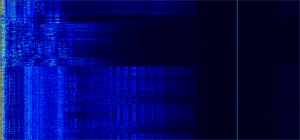
At this point, we almost have an audio signal. Lets have a look at it:

The lower part of the spectrum from 0 to the weird red line kinda looks like an audio spectrum. The red line is actually a strong tone at 19KHz. Then, after the red line there is another signal. This is actually where the stereo information is encoded.

The tone at 19KHz indicates the presence of the stereo signal and the symmetric signal centered on 38KHz (twice 19KHz) is a double sideband suppressed carrier AM (yes - this is AM modulation on top of FM modulation) signal representing the difference between the left and right channels. To decode the stereo signal, we start with the mono audio signal below 19KHz and add this AM signal to one channel and subtract it from the other.

What’s cool about this is that old FM receivers that were designed before this stereo encoding was standardised would still continue to function with the stereo signal. They all probably filtered out audio signal above 19KHz since that is above the range of most human hearing, and, if they didn’t, the listener would not have been able to hear it anyway, unless they were a dog.

To keep things simple, we wont actually decode the stereo signal in this blog post, but its interesting to see the signal nonetheless.

Resampling

Before we output our sound signal to out speakers, we must resample it so that its sample rate matches what our sound card expects. 48KHz is a commonly supported frequency for sound cards. Our current sample rate is 160KHz. To make it 48KHz, we need to resample it down by a factor of 3/10 using the firResampler pipe.

Doing this, and again outputting the frequency spectrum:

let coeffsResp :: [Float]
	coeffsResp =  VS.toList $ windowedSinc 85 0.25 blackman
resp <- lift $ fastResamplerR cpuInfo 3 10 coeffsResp

lift $ runEffect $   
        str 
    >-> P.map (interleavedIQUnsignedByteToFloatFast cpuInfo :: VS.Vector CUChar -> VS.Vector (Complex Float)) 
    >-> firDecimator deci fftSize
    >-> firDecimator deci fftSize
    >-> firDecimator deci fftSize
    >-> fmDemod
    >-> firResampler resp fftSize
    >-> P.map (VG.zipWith (*) window) 
    >-> P.map (VG.map float2Double)
    >-> audioFFT
    >-> P.map (VG.map ((* (32 / fromIntegral fftSize)) . double2Float . magnitude)) 
    >-> audioSpectrum

Now that our sampling frequency is 48KHz, most of the spectrum is occupied by the audio signal. We still have that pesky 19KHz pilot tone. Fortunately, we can easily get rid of this with a filter just as we did to the original spectrum at the beginning of the post.

Playing the audio

Finally, we have a pure audio signal at the correct sampling rate. We pipe it to our speakers using the pulse audio sink….

audioSink <- lift pulseAudioSink

lift $ runEffect $   
		str 
	>-> P.map (interleavedIQUnsignedByteToFloatFast cpuInfo :: VS.Vector CUChar -> VS.Vector (Complex Float)) 
	>-> firDecimator deci fftSize
	>-> firDecimator deci fftSize
	>-> firDecimator deci fftSize
	>-> fmDemod
	>-> firResampler resp fftSize
	>-> firFilter filter fftSize
	>-> audioSink

..and we get surprisingly high quality audio playing from our speakers.